I’ve just passed my intermediate amateur radio exams with the help of Stockport Radio Society G8SRS. I’ll be keeping my previous call-sign M6TKG for now, but I’ll also now be using 2E0TKG under certain circumstances. As a gift to myself for passing, I’ve started putting together a little portable rig for low-power (QRP) work based on a Yaesu FT-817ND. I’ve already started reading for my full licence test, and have just begun working towards my 12 words-per-minute Morse code test. I hope that soon I’ll be in a position to bring a rig away when I travel, and make some contacts from some of the unusual places I sometimes have the opportunity to visit.
High-resolution proglacial lake records of pre-Little Ice Age glacier advance, northeast Greenland
I’m pleased to announce that a paper I was involved in (led by colleagues from Manchester Metropolitan University and Liverpool John Moores University) has now been published in Boreas. The paper presents a record of glacial activity in Greenland over centennial time-scales using lake sediment geochemical proxies. My contribution was in the multi-variate statistical treatment of the elemental data, alongside some modelling work on the chronology. The paper is available online here.
Technicians Make it Happen Profile
The Gatsby Charitable Foundation runs a campaign called Technicians Make it Happen, raising the profile of technicians in the U.K. It’s been supported by the Science Council, amongst others, and I’m glad to be a part of the campaign this week with my profile being published on their website.
Bicycle Distance Sensor
Introduction
A student recently came to us with a project that would make use of Dr Ian Walker’s bicycle overtaking sensor, so I agreed to make him one. Since Dr Walker published his original article, the code has had to change a bit, so I thought this would be a good opportunity to post the updated code and include a complete bill of materials.
Bill of Materials
- Arduino Uno rev.3, e.g. RS #715-4081
- Adafruit datalogging shield #1141 (I purchased from Pimoroni)
- Button battery, CR1220, e.g. CPC #457-4713
- header pins, 2.54 mm, e.g. CPC #CN18415
- SD card, e.g. Transcend TS2GSDC, e.g. RS #758-2552
- M3 self-tapping screws, 4 mm, e.g. RS #500-5094
- Sellotape Sticky Fixers, e.g. CPC #OE02909
- jumpers, e.g. CPC #SC12901
- heat shrink tubing, 3:1, 3.2 mm diameter, e.g. CPC #CB10468
- Maxbotix ultrasonic sensor (either a MB1200 XL-MaxSonar EZ0, or an EZ2); I bought from Cool Components (stock numbers #484 or #595 respectively)
- M3 standoffs, 6 mm, e.g. RS #222-373
- 4-way socket, e.g. CPC #CN14906
- 4-way plug, e.g. CPC #CN13577
- 4-way cable, e.g. RS #660-7067
- Power switch, e.g. RS #314-4995
- Crimp connectors, e.g. CPC #4217251
- Push button switch with light, e.g. RS #457-4713
- 3-d printed enclosure for the switch (click to download my *.stl file that fits the switch above)
- Bicycle flashlight holder, e.g. this item from eBay
- cable ties, 2.5 mm, e.g. CPC #CBBR6667
- AAA battery holders x2, e.g. RS #512-3552
- Enclosure, I used a Hammond 1591ESBK, e.g. RS #415-2846
Code for Arduino
You’ll need a USB cable to program the Arduino. I have made some modifications to Dr Walker’s original code. They address four points:
- The RTC (real-time-clock) used in the latest revision of the Datalogging Arduino Shield has changed. This addresses the changes needed.
- There is a new library available for the Maxbotix distance sensors which is a far more elegant than the old alternatives.
- I’ve decided to use the internal pull-up resistor on the button input, rather than an external pull-down. It saves on the wiring!
- I’ve added a serial output for checking the unit is working correctly.
The revised code is available here. Remember that the first time you use the RTC, you need to program it – instructions can be found here.
Building the Unit
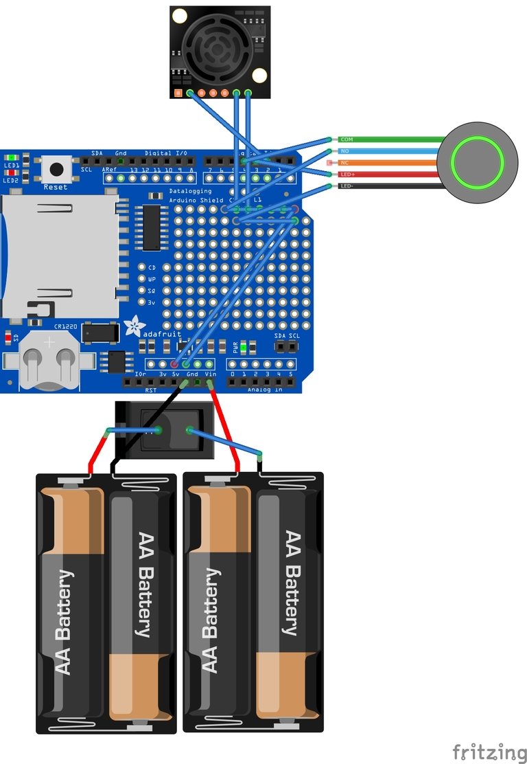
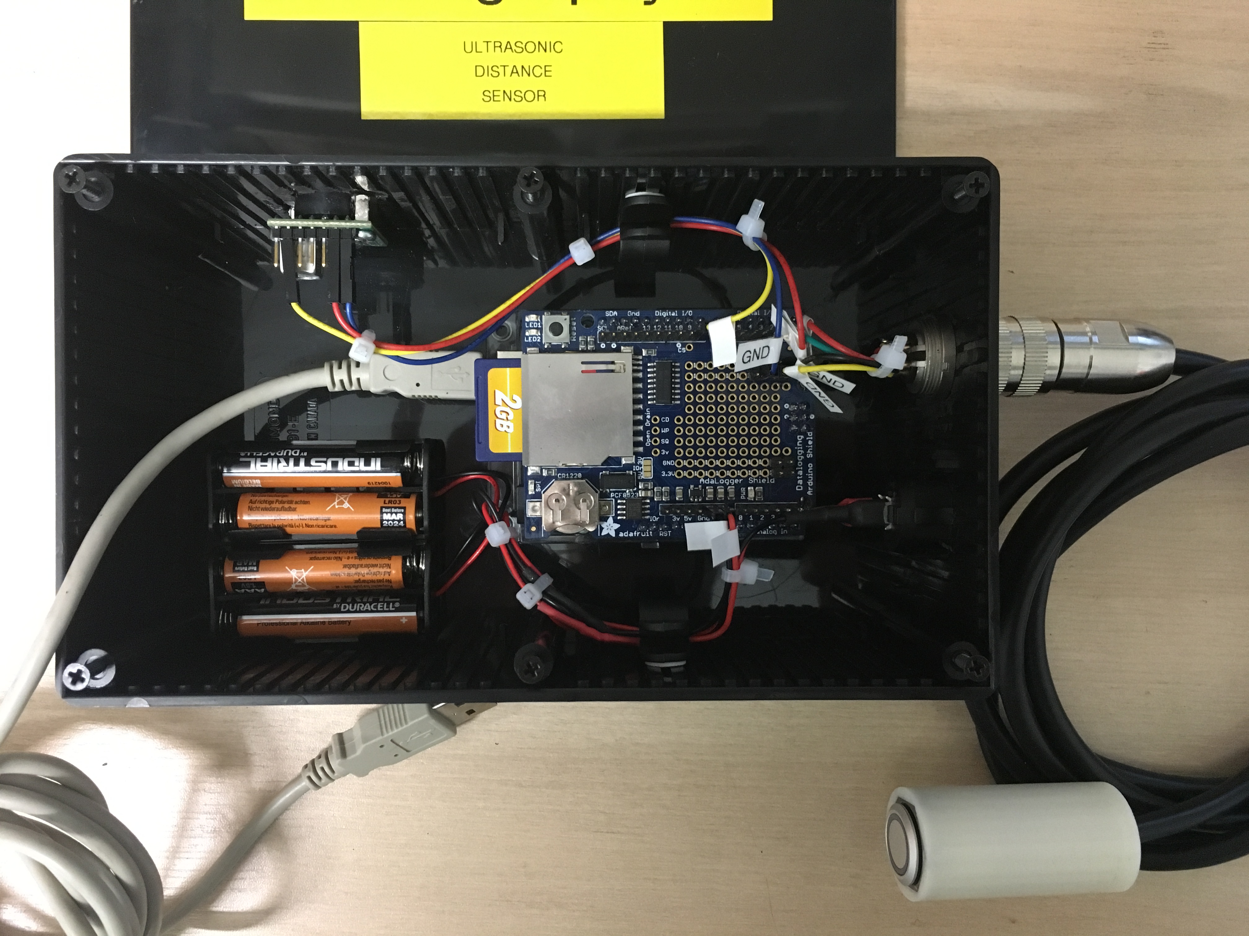
It should be pretty obvious how this all goes together from the photographs, code and wiring diagrams, but a few hints:
- The handlebar button fits in the printed enclosure, and the cable can be secured with a cable tie to stop it pulling on the button connections. A tiny dab of super-glue holds the button in place.
- The Arduino and shield can be secured using the base plate that comes with all Genuino’s using the self-tapping screws, and the base plate secured in the enclosure using the sticky fixers.
- I secured the Maxbotix sensor to the enclosure by screwing two standoffs to it, and gluing the standoffs to the inside of the enclosure.
- I thought it easier to connect the power button using crimp connectors. This allowed me to easily fit the button to the enclosure. The battery holders are held down with sticky fixers.
Conclusions
I’ll update this section in due course when we have the results of the research conducted with this sensor!
Rescaling for Compression
Sometimes when coring, cores can become compressed in the chamber. For example, if you know you’ve started a drive at 1 m, and finished at 2 m, but only collected 0.95 m of sediment, you may have compression. This is often a problem for Livingstone-type corers, but not an issue with Russian-types. This can be caused by:
- stretch in locking lines for corer heads (or ground compression if those lines are locked to the surface),
- friction of sediment inside the tube,
- airlocks inside the tube,
- poor cutting performance of the corer end.
It’s difficult to know whether you’ve lost material or suffered compression, so good practice says the stratigraphy should be cross-correlated with an adjacent sequence. If there is compression, this can be corrected for, but in practice it can be a pain. Here’s a simple way of doing it in R. Here I’m correcting the depths for sub-samples taken at 10 mm intervals, in a core that should have been 1 m in length, from 1 m to 2 m depth, but was actually 0.95 m in length when extracted.
length <- 950     # the measured length of the core when extracted
truestart <- 1000 # the starting depth of the drive
trueend <- 2000   # the finishing depth of the drive
intervals <- 10   # the sampling interval

# create the sampling sequence - this may already be available in your data
z <- seq(from = trueend-length, to = trueend, by = intervals)

# correct those depths
zc <- seq(from = truestart, to = trueend, length.out = length(z))

# compare the data
df <- data.frame(original = z,
                 corrected = round(zc, digits = 0),
                 difference = round(z-zc, digits = 0)
                 )
head(df)
tail(df)
This code assumes that there’s more compression at the top, and less at the bottom of the sequence, which is not unreasonable given the possibles causes listed above. Sometimes cores can expand due to decompression of the sediment following coring. This is particularly common in gytjja from lakes, where the weight of the water column compresses the sediment in-situ, thus it expands ex-situ. Take an example where we have a core of length 1.05 m, but we know we only cored from 1 m to 2 m; we need to compress the core back to 1 m length. The following code deals with this problem:
length <- 1050    # the measured length of the core when extracted
truestart <- 1000 # the starting depth of the drive
trueend <- 2000   # the finishing depth of the drive
intervals <- 10   # the sampling interval

# create the sampling sequence - this may already be available in your data
z <- seq(from = truestart, to = truestart+length, by = intervals)

# shift the depths so they are centered
zs <- z-(max(z)-trueend)/2

# correct these depths
zc <- (trueend-truestart)/length * zs + mean(c(trueend, truestart)) - ((trueend-truestart)/length) * mean(zs)

# compare the data
df <- data.frame(original = z,
                 shifted = zs,
                 corrected = round(zc, digits = 0),
                 difference = round(zs-zc, digits = 0)
                 )
head(df)
tail(df)
Official New Divisions for the Holocene
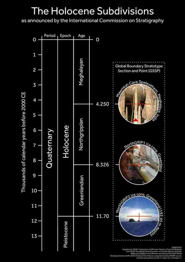
It’s official! The I.C.S. have announced the subdivisions for the Holocene, so I’ve made a helpful graphic to summarise their announcement, which I’ve reproduced in full below.
Formal subdivision of the Holocene Series/Epoch
It has been announced that the proposals for the subdivision of the Holocene Series/Epoch (11 700 years ago to the present day) into three stages/ages and their corresponding subseries/subepochs by the International Subcommission on Quaternary Stratigraphy (ISQS) (a subcommission of the International Commission on Stratigraphy – ICS) have been ratified unanimously by the International Union of Geological Sciences (IUGS). The subdivisions now formally defined are:
1. Greenlandian Stage/Age = Lower/Early Holocene Subseries/Subepoch
Boundary Stratotype (GSSP): NorthGRIP2 ice core, Greenland (coincident with the Holocene Series/Epoch GSSP, ratified 2008). Age: 11,700 yr b2k (before AD 2000).2. Northgrippian Stage/Age = Middle/Mid-Holocene Subseries/Subepoch
Boundary Stratotype (GSSP): NorthGRIP1 ice core, Greenland. Global Auxiliary Stratotype: Gruta do Padre Cave speleothem, Brazil. Age: 8326 yr b2k.3. Meghalayan Stage/Age = Upper/Late Holocene Subseries/Subepoch
Boundary stratotype (GSSP): Mawmluh Cave speleothem, Meghalaya, India. Global Auxiliary Stratotype, Mount Logan ice core, Canada. Age: 4250 yr b2k.These divisions are now each defined by Global Stratotype Sections and Points (GSSPs), which means that they are fixed in time in sedimentary sequences. The terms Greenlandian Stage/Age, Northgrippian Stage/Age, Meghalayan Stage/Age, Lower/Early Holocene Subseries/Subepoch, Middle/Mid-Holocene Subseries/Subepoch and Late/Upper Holocene Subseries/Subepoch therefore have formal definitions and boundaries.
These definitions represent the first formal geological subdivision of the Holocene Series/Epoch, resulting from over a decade of labour by members of the joint ISQS (International Subcommission on Quaternary Stratigraphy) – INTIMATE Members Working Group (Integration of Ice-core, Marine and Terrestrial Records), led by Professor Mike Walker (University of Aberystwyth).
Phil Gibbard
Secretary General ICS
Cambridge 26.6.18
Fake Morgan Dollar & Pound Coin – Metallurgy
The Morgan silver dollar is a precious metal coin minted in the late 19th century into the early 20th century. They are collectable and thus occasionally counterfeited. I’ve recently analysed genuine and counterfeit silver dollars using x-ray fluorescence (XRF) – here I’ve used a Rigaku NEX-CG ED-XRF instrument using a “fundamental parameters” estimation mode. There’s some work to do to optimise the system for these samples – it’s not something we usually work on!
Anyhow, the counterfeit seems to be brass, plated with silver. The real thing has a specification of 90% Ag, 10% Cu.
| Element | Specification | Genuine | Counterfeit |
| Ag | 90 % | 92.3 % | 27.2 % |
| Cu | 10 % | 6.6 % | 43.1 % |
| Zn | 0 % | 0.0 % | 26.0 % |
I’ve also analysed some old “round-pound” £1 coins. These were demonetised in 2017, because nationally around 1 in 30 of the coins in circulation were counterfeit – I’ve heard that in some areas, the number could have been as high as 1 in 5. I’ve found that genuine and counterfeit coins have a pretty similar Nickel-Brass metal, but can be easily distinguished by their Pb content – around 1.5 % in counterfeits, and negligible in genuine coins. The Pb is added to improve malleability.
| Specification | Genuine (1 σ, n = 8) | Counterfeit (1 σ, n = 2) | |
| Ni | 5.5 % | 6.0 ± 0.5 % | 4.9 ± 0.1 % |
| Cu | 70.0 % | 69.9 ± 0.6 % | 67.3 ± 0.4 % |
| Zn | 24.5 % | 23.1 ± 0.9 % | 25.1 ± 0.1 % |
| Pb | 0.0 % | 0.0 ± 0.0 % | 1.4 ± 0.6 % |
I’m going to develop this into part of an outreach activity that uses our Niton Handheld XRF. I’m planning demonstrations of contaminated vs. uncontaminated soils, and some other geological samples.
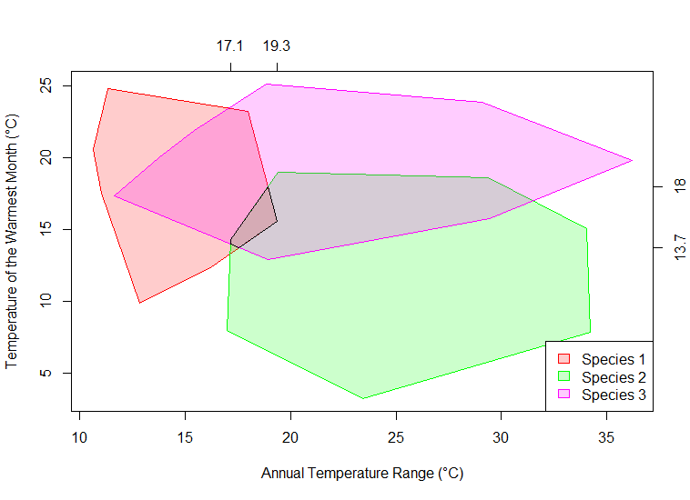
Illustrating the Mutual Climate Range (MCR) Method
I’m writing up some lecture material on transfer functions and environmental reconstruction, and needed to draw a diagram to illustrate the mutual climatic range method. This code could also be used to make simple MCR calculations and the like.
Tyre Depth Gauge for Loose Powder XRF Preps
When we prepare samples for analysis by XRF we tend to use a simple pressed powder preparation method in the first instance. The depth of the sample is important for calculating matrix density and in correcting for non-infinite depth samples (thin samples and/or those with a low average atomic number). We used to use a standard digital caliper, but it wasn’t ideal. The 150 mm calipers we had were unwieldy, and it care was needed to accurately level the depth gauge probe.
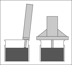
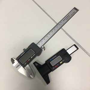
Enter the digital tyre depth gauge! These digital tyre depth gauges are easy to find online for a few quid. They have a nice wide guide, and as you can see with a range of up to 25 mm, they are perfect for measuring the depth in XRF loose-powder pots (we use pots that are nominally 22 mm tall). The method goes:
- Zero the display whilst measuring the depth of the empty pot.
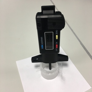
Measure from the top of the pot to the base, and zero the display. - Fill the pot with sample, press and weigh.
- Measure to the top of the sample from the top of the pot.
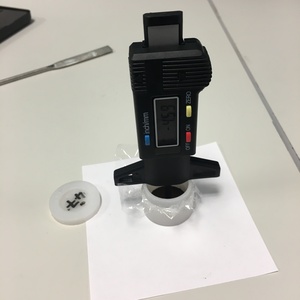
Having filled the pot with the sample, probe from the top of the pot to the sample surface. - The height of the sample is the additive inverse of the reading (that is, -7.45 mm is 7.45 mm).
How The Itrax Core Scanner Works – New Poster
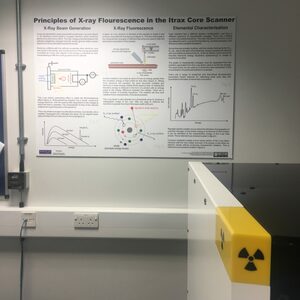
Having described the basic mode of operation of the Itrax core-scanner countless times in the past few months, I thought it time for a proper poster with nice diagrams, so I recently made this poster for the Itrax facility I’m looking after. It has a description of how x-ray beams are created and controlled in the scanner, the principles of measurement, and an explanation of how deriving chemical compositional data from fluorescence spectra can be done. It’s available from the resources page of this website. Let me know if you print one and use it – I love seeing photos of resources I’ve created being used!
If you need more information on the Itrax core scanner, there’s this paper and this edited volume that may be of interest.
