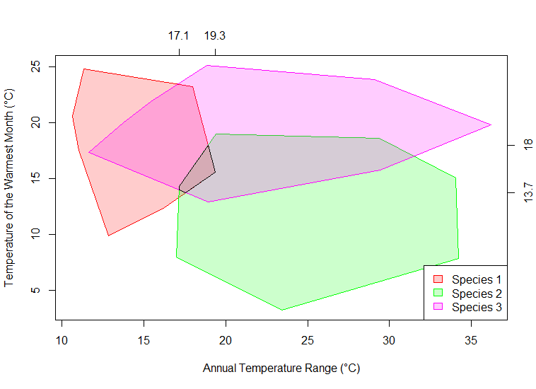
I’m writing up some lecture material on transfer functions and environmental reconstruction, and needed to draw a diagram to illustrate the mutual climatic range method. This code could also be used to make simple MCR calculations and the like.

# create 3 sets of normally distributed data

x1 <- rnorm( 100, 15, 2   )

y1 <- rnorm( 100, 19, 2.5 )

#

x2 <- rnorm( 100, 25, 4 )

y2 <- rnorm( 100, 12, 3 )

#

x3 <- rnorm( 100, 25, 5 )

y3 <- rnorm( 100, 20, 2 )

#

# compute the convex hull of those data

h1 <- c( chull( x1, y1 ), chull( x1, y1 )[ 1 ] )

h2 <- c( chull( x2, y2 ), chull( x2, y2 )[ 1 ] )

h3 <- c( chull( x3, y3 ), chull( x3, y3 )[ 1 ] )

#

# this library deals with polygon clipping

require( polyclip )

#

# compute the clipping area

# this is a polyclip method inside another polyclip method

# because polyclip is pairwise

clip <- polyclip( polyclip( list( x = x1[ h1 ],

y = y1[ h1 ] ),

list( x = x2[ h2 ],

y = y2[ h2 ] )

),

list( x = x3[ h3 ], y = y3[ h3 ] )

)

#

# plot the polygons

plot( 0,

type = "n",

xlim = c( range( c( x1, x2, x3 ) ) ),

ylim = c( range( c( y1, y2, y3 ) ) ),

xlab = "Annual Temperature Range (°C)",

ylab = "Temperature of the Warmest Month (°C)"

)

polygon( x1[ h1 ], y1[ h1 ], col = adjustcolor( "red", alpha.f = 0.2 ), border = "red" )

polygon( x2[ h2 ], y2[ h2 ], col = adjustcolor( "green", alpha.f = 0.2 ), border = "green" )

polygon( x3[ h3 ], y3[ h3 ], col = adjustcolor( "magenta", alpha.f = 0.2 ), border = "magenta" )

polygon( clip[[ 1 ]] )

#

# add a legend

legend( "bottomright",

legend = c( "Species 1", "Species 2", "Species 3" ),

fill = c( adjustcolor( "red", alpha.f = 0.2 ),

adjustcolor( "green", alpha.f = 0.2 ),

adjustcolor( "magenta", alpha.f = 0.2 )

),

border = c( "red", "green", "magenta" )

)

#

# mark the mutual ranges on the opposing axes

axis( 3,

labels = round( c( min( clip[[ 1 ]]$x ),

max( clip[[ 1 ]]$x ) ),

1 ),

at = c( min( clip[[ 1 ]]$x ),

max( clip[[ 1 ]]$x) )

)

axis( 4,

labels = round( c( min( clip[[ 1 ]]$y ),

max( clip[[ 1 ]]$y ) ),

1 ),

at = c( min( clip[[ 1 ]]$y ),

max( clip[[ 1 ]]$y) )

)