Simple Single Ring Constant-head Infiltrometer

Here’s how to make a very simple single ring constant head infiltrometer – it could be particularly suitable for school projects at key-stage 4 or 5. Commercially available double-ring infiltrometers with a Mariotte’s bottle would be more suitable for research purposes, but these can be surprisingly expensive.

How To Make It

You’ll need:

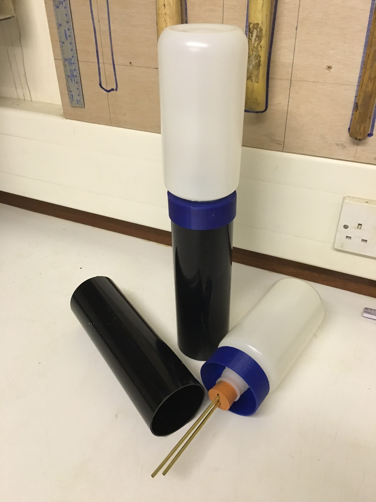
A piece of downpipe (I’ve used 68mm PVC pipe)
A bottle (I’ve used a Nalgene #2089-0032 1l bottle)
A rubber bung to fit the bottle (I’ve used a BS2775 #25)
Two brass tubes (c.4mm ID)
Access to a 3D printer (or use a 3D printing service) to print the adaptor
A tube of 2-part epoxy (I’ve used Araldite #ARA-400007)
A drill and some c.4mm drill-bits
A stopwatch

Drill two holes in the bung to fit the brass rods, and insert them. Measure the bottle and the downpipe and design and print an adaptor (or use/adapt the 3D model from here). The adaptor is entirely optional – it is only there to neaten things up and allow hands-free operation. Now glue the adaptor onto the bottle using the two-part epoxy, put the bung/pipe assembly in, and fit on-top of the downpipe. You should also drill a small hold into the downpipe just below the adaptor fitting to act as a vent. You will need to put calibrated marks on the bottle in order to measure volume – I suggest filling the bottle and decanting into a volumetric flask, marking e.g. every 10ml.

How to Use It

To use, push the downpipe about 5cm into the sediment, and adjust the brass pipes so one is 10mm from the soil surface, and the other slightly more (perhaps 13mm). Fill the bottle, fit the assembly onto the downpipe and immediately start a stopwatch. Record the water level at regular time intervals appropriate to the rate of flow – this might take some experimentation. Remember to carry a supply of extra water! The data should be processed to convert it to flux, in cubic meters per second. Typically the flux will stabilise after some time – the flux at which it stabilises is referred to as the “(quasi-)steady-infiltration rate”.

How to Process the Data

The aim is to establish a soils hydraulic conductivity, or “field-saturated hydraulic conductivity”, expressed as $K_{fs}$ . There are two main groups of equations that can be used: those that recognise the lateral flow, and those that only recognise the vertical flow. I’ll illustrate a couple of simpler models here, but check the references below for detail of the theory and limitations. Both the examples given here require the steady-infiltration rate mentioned above.

Simplified Method

$K_{fs}=Q_{s}$

Where $K_{fs}$ is the field saturated hydraulic conductivity, in m/s, and $Qs$ is the (quasi-) steady infiltration rate in m³/s. This method assumes one-dimensional, vertical flow and is known to over-estimate conductivity; see Reynolds et al. (2002) for a fuller appraisal.

Bouwer Method

$K_{fs}=\frac{Q_{s}}{\frac{H}{L_{f}}+\frac{1}{\alpha^{*}L_{f}}+1}$

Where $L_{f}$ is the depth from the infiltration surface to the wetting front in meters (or, the depth of soil), $H$ is the water height in meters, and $\alpha^{*}$ is the macroscopic capillary length parameter in m^-1 (Bouwer, 1966, 1986). Choosing a value of $\alpha^{*}$ is important but can be difficult; in the table below I’ve paraphrased some common values from Reynolds et al. (2002) , table 2.4-4 (p.820).

Soil Type	$\alpha^{*}$ (m^-1)
Compacted, unstructured, clayey or silty materials e.g. lacustrine or marine sediments, landfill caps.	0.0001
Fine textured, unstructured soils (clayey or silty). Also fine sands.	0.0004
Most structured soils from clays to loams, unstructured medium to find sands. Most frequently used for agricultural soils	0.0012
Coarse and gravelly sands, or highly structured, largely cracked, or aggregated soils, or soils with macropores.	0.0036

Some main sources of error are:

that the small sample area may not be representative of the study area
- this could be tempered by taking a number of measurements across the study area and making an appraisal of the consistency of otherwise of the results
the soil is disturbed by the insertion of the infiltrometer ring
- this is largely unavoidable, but some care can be taken to gently insert the rings, and to ensure they aren’t jostled or wiggled as they are handled
that there is edge flow that causes an over-estimation of the hydraulic conductivity
- edge flow is when water takes a “shortcut” by running along the side of the infiltrometer ring wall.
the model used in calculating hydraulic conductivity is insufficiently accurate
- there are a range of models – see for example the work of Reynolds, Wu or Young’s as alternatives to the simpler models presented above.
- the assumptions of the model cannot be met. For example, ponding of water outside the ring is incompatible with some models.