Tom Bishop: Lab Notes

You may be familiar with the classic GRADISTAT for calculating particle size statistics. It is a set of macros written into a Microsoft Excel spreadsheet by Kenneth Pye and Simon Blott. At the time of writing it was last updated for use with Microsoft Excel 2007, and is becoming increasingly difficult to use with newer versions of Excel. After recently troubleshooting some odd GRADISTAT outputs for one of our lab users, I decided to see if there were alternatives available.

G2SD, written by Regin Gallon and Jerome Fournier, does everything GRADISTAT did and a little more, and all as an easy to use package in R. Easy to use R? I hear you ask! Well yes, because it has the option of using a web-based interface (built using the “shiny” R package). I’m (very) still starting out with R, and I’m not finding it easy! However, this package can be used with minimal knowledge – just follow my instructions below. Want to try it out first, or only need basic functionality? Why not use the hosted web-based version, available here for use with delimited text files (e.g. *.csv, *.tab).

Install R and G2Sd

1. Assuming you are a Windows user, visit the R website, download and run the installation file, selecting the default options.
2. Visit the repository for G2Sd and download the latest stable version.
3. Open RGui, and from the top navigation menu, select Packages>Install Packages From Local Files.
4. Navigate to the downloaded *.zip file that contains G2Sd files.
5. G2SD is dependent on some other packages. Install the first by typing install.packages(“shiny”).
6. Repeat step five but replace shiny with xlsx, then rJava, xlsxjars, reshape2 & ggplot2.
7. You only need to do this once!

Loading and Using G2Sd

1. Load G2Sd by typing library(G2Sd), or by navigating Packages>Load Packages>G2Sd from the top navigation menu.
2. Run the web browser based GUI by typing granstat(web_interface=TRUE). A web-browser should appear!
3. The data should be in the format:
   1. The first column are the sieve mesh sizes in microns, in descending order (from largest to smallest aperture). Size “0” is the pan.
   2. Columns subsequent to the first are a sample. The first row is the sample identifier.
4. From here you can visualise and download the data.

Using the Command Prompt Instead

1. Load G2Sd as previously described.
2. Load CSV data into an R dataframe by typing mydata <- read.table(“mydata.txt”, header=TRUE, sep=”,”). If you don’t have your own data, an example dataset is included in the package. Try loading it using data(granulo), and exporting it to a CSV datafile using write.table(granulo, “granulo.txt”, sep=”,”).
3. For statistics, try typing granstat(mydata). There’s a lot more functionality here – check out the package documentation for more.
4. If you want to export these to a CSV file, just combine the two functions we met previously: type write.table(granstat(mydata), “mydata.txt”, “sep=”,”).
5. For graphics, try trying grandistrib(mydata). There’s options for multiple samples to be plotted, and a number of different styles – try granplot(mydata) or granplot(mydata, xc=2:4) for a couple of examples. Check out the package documentation for more.
6. To export a graphic generated in the data frame, right click the figure and save using the dialog box.

References:

Blott, S.J. & Pye, K. (2001). “GRADISTAT: a grain size distribution and statistics package for the analysis of unconsolidated sediments”. Earth Surface Processes and Landforms v26, pp.1237-1248.

Fournier J., Gallon R. (2014). “G2Sd: a new R package for the statistical analysis of unconsolidated sediments”. Géomorphologie : relief, processus, environnement v20(1), pp.73-78.

 

I’ve hooked up one of our lab balances to a PC!

For users of the Geography Laboratory

In the main lab is a networked computer that I’ve connected to the Ohaus Adventurer AR-Series balance. To use it:

• login
• open “C:\SPDC Data Collection V2.01\SPDC Data Collection V2.01.exe”
• click “Browse”, find the Excel spreadsheet you want to import to, and click “Open”
• click “Run”. It will automatically open the spreadsheet and connect to the balance
• select to cell you want to populate, and press the “Print” button on the balance; it will populate the cell with the current reading.

How’s it Done and Can You Do This With Other Balances?

Almost all laboratory balances have RS232 communications built in as standard, but for some reason they seem to want to make it as hard as possible to use them! This is unfortunate, because this functionality is really handy for connecting them up to spreadsheet packages like Excel for automatic data entry. If you can get it working, it is an easy way to save all your lab users time and reduce transcription errors. I’ve had a good hack at the Ohaus balances in our lab, and here are some notes on my experiences. My next project will be to pipe these serial connections over IP, and then allow access via a WIFI hotspot. Just connect to the WIFI hotspot, start the wedge software and measure away – well that is the plan, anyway.

Ohaus Adventurer AR-Series (like above)

These should be straightforward – they have configurable Rs232 communications and a standard male DB-9 connector. Of course, for reasons best know the the manufacturer, they have completely non-standard pin assignments. The pin assignments are shown in the manual, so you’ll have to build your own null modem cable to connect it, or the ground ends up connected to the CTS and you get nonsense. On the plus side, Ohaus supply the wedge software for free, which will allow direct input into a .xlsx, .csv, etc. The standard serial settings are 2400 7N2 (yeah, why not?), but these are configurable so you could change them to something this side of sensible (like 9600 8N1). Once it is all up and running, just press “print” to fill a cell.

Ohaus Explorer (& Pro)

Now here’s a thing: although the pin assignment and default serial settings are the same as for the Adventurer series, the RTS/CTS is implemented differently. No problem, just set the correct flow control in the wedge software, right? Well, we would if we could, but the Ohaus wedge software doesn’t implement hardware handshaking properly! Open a serial connection using Minicom or PuTTY and you’ll have no trouble sending and receiving (when you configure the handshaking properly), but try the Ohaus software, and it won’t play. You’ll have to tie the CTS and DTR pins together to get them to work – it’s a bit ham-fisted, but it’ll do. This will be my next project.

Mettler Toledo 

Naturally, Mettler Toledo fit a serial interface without the familiar DB-9 connector. I’m working on sourcing it, but I suspect it’ll be £££.

Sartorius

Haven’t started on these yet, because we don’t have many in the labs, although previous experience tells me they are usually good at implementing serial comm’s over RS-232.

I’m on GitHub! At the moment I’m using it to develop, update and distribute the LaTeX templates for typesetting theses, associated with the courses I deliver on the subject. Expect the addition of some of the Python-based dGPS, ADS-B and other radio-science scripts I’ve written.

If like me you’ve been experimenting with Raspberry Pi’s you’ll know putting monitors, mice and keyboards costs far more than the units themselves and presents some difficulty. Not just that, but running “headless” systems is normally preferable for the kind of applications I’m working on (servers, radios, desktop gadgets). If you can get away with only hooking up KVM (keyboard, video, mouse) once (or not at all!), great! There’s loads of guides knocking around, but here’s how I do it:

Using a KVM

First, I connect the Pi to the telly with a spare HDMI connection, plug in a wireless mouse and keyboard and run NOOBS to install Raspbian. I assume the systems are on the same local network, so use hostnames here. If you are connecting over the internet, you’ll need to replace these with a public IP or domain name.

Using the Serial Interface

First I connect a Raspian image onto SD and connect up a TTL serial interface (find the pinouts for your Pi). Use Device Manager to find the COM number of the interface on your PC, then use PuTTY to configure it (the baud is 115200) and connect to a session on the Pi. Use the default logins and follow the instructions below.

Enable SSH

First I run sudo raspi-config and enable SSH and change the hostname. I choose not to reboot, but quit raspi-config and run sudo shutdown now. Now, simply login from Windows from PuTTY using the hostname and default settings. Using the hostname avoids the need to assign a static IP.

Enable RDP

If you want a desktop, RDP is built into Windows 10 and is an easy way to remote into the x-window system, all you need to do is install xrdp. Just install like any other package (sudo apt-get install xrdp). Now reboot the Pi and find the Remote Desktop Connection client on your Windows 10 system, and enter the hostname to connect.

Security

Remember, by opening up remote access servers like these, you open the Pi up to potential attacks, especially if you have external access from the internet. Internal attacks might not be a big problem on your internal network, but if you choose to open these up over the net, think about using random port numbers, public/private keys and tunneling the RDP over SSH.

I’ve been experimenting with a Raspberry Pi B v3, which has an onboard bluetooth radio. I’ve been interested in using GPS (or more correctly, GNSS) radio receivers with the Raspberry Pi for a while now, but the price of development platforms for the Raspberry Pi is quite high. I dug out a bluetooth GPS receiver from a box of old electronics, and found it surprisingly easy to connect to. I think I’m still going to have to invest in a proper development board at some point because the bluetooth GPS lacks a pulse-per-second (PPS) output with I’d like to use to build a stratum-1 NTP server, but for now, here’s how I got the GPS working:

Connecting to the Bluetooth Device

The program bluetoothctl can be used to control the bluetooth radio on the Pi. To connect to a bluetooth device, follow these steps:

• use the command bluetoothctl at the CLI. This opens the program. Try the command help to see a list of possible commands.
• power on
• scan on – find and note the target mac address from the list
• agent on
  • error message? Try:
    • select YO:UR:MA:CA:DD:RE:SS:00
    • default-agent
    • agent on
• pair DE:VI:CE:MA:CA:DD:RE:SS & enter code if required
• trust DE:VI:CE:MA:CA:DD:RE:SS (if you want to skip confirming trust in future)
• exit (to exit)

Connecting to the Bluetooth Serial Interface

We use the program RFCOMM to connect to the bluetooth serial interface. First, load it with the command “sudo modprobe rfcomm”. Now connect (or “bind”) the GPS receiver to the RFCOMM “device” using “rfcomm bind rfcomm0 DE:VI:CE:MA:CA:DD:RE:SS”. Note that the connection will only be initialised when a program attempts to open the RFCOMM device.

Checking the State of the NMEA Messages

Most GPS units will communicate using messages sent in ASCII over a serial data connection. The format is standardised with the NMEA0183 specification, with compliance highly variable! Most receivers have the same serial communications settings – 4800 baud 8N1 (that is, data bits=8, parity=none, stop bits=1, handshake=none). You can use Minicom in Unix-like system (or PuTTY in Windows) to view the messages as they arrive. On the Raspberry Pi, you could use minicom – or you could skip directly to GPSD to probe the messages sent by the GPS.

To use minicom, you need to install it (sudo apt-get install minicom) and then open the configuration menu (minicom -s). Select “configure serial port” and give it the NMEA standard settings above. Set the serial device to “/dev/rfcomm0”. Save the setup as the default, exit, and start the program (minicom). You should see the messages as they come in! Remember to exit it’s the intuitive (!) CTRL+A then X.

You might also use GPSD, a program designed to utilise GPS devices in a number of ways. One of the best things about GPSD is that it automatically detects and configures the connections, so you don’t have to tell it what kind of serial connection you need or what messages to expect. It does need to know to look for the bluetooth connection though, so…

• Install using “sudo apt-get install gpsd gpsd-clients python-gps” (ok, there’s some extra bits there for later…)
• a bit of housekeeping to avoid some conflicts in manually run instances (sudo systemctl stop gpsd.socket, then sudo systemctl disable gpsd.socket)
• sudo gpsd /dev/rfcomm0 -F /var/run/gpsd.sock to connect the rfcomm0 device to the GPSD socket, and
• gpsmon to open the program that both parses the position data and displays the messages as they arrive.

What do these messages mean? I won’t go through them all, not least because the specification is not freely available, but also because there are all sorts of different messages. A bit of Google-fu might be required if you see something unusual, although the document IEC 61162-1 is very closely derived from NMEA0183 and you may have easier access to this document. A GPS unit will output a number of lines, cycling through them; for example, mine outputs a RMC, VTG, GGA, GSA x5 times over, then GSV spread over four lines then repeat.

• RMC contains the “minimum recommended data for GPS”
• VTG contains “velocity made good” speed and heading information,
• GGA contains essential fix data including quality indicators
• GSA contains GPS dilution of precision and information on satellites in use
• GSV contains information on the satellites that could be in use based on available data – this is often spread over multiple lines

$GPGGA,161229.487,3723.2475,N,12158.3416,W,1,07,1.0,9.0,M, , , ,0000*18

• $ defines the beginning of the message
• GP is the “talker ID” and identifies the type of unit that is sending the message. This is sometimes programmable, but is always two letters, most commonly GP for generic GPS
• GGA defines the type of message the follows – this is always three letters. Here, GGA means the message is a “Global Positioning System Fix Data” message. This defines what the following commas separated values are:
• 161229.487 is the UTC time in hhmmss.sss format
• 3723.2475 is the latitude in decimal degrees, in the format ddmm.mmmm
• N refers the hemisphere of the latitude, north or south
• 12158.3416 is the longitude in the same format as the latitude
• W is the hemisphere of the longitiude, east or west
• 1 defines whether the signal is valid and whether it is from a standard or differential fix
• 07 is the number of satellites used to calculate the fix
• 1.0 is the horizontal dilution of precision – or the accuracy in the x and y plane
• 9.0 is the altitude above mean sea level
• M is the units (here, meters) of the altitude above mean sea level
• the next three fields are blank, as they refer to parameters for differential fixes
• 0000 is a null value as it refers to a parameter for differential fixes
• * defines the end of the message
• 18 is a checksum for error-checking the previous message, and may or may not be present

There are messages that give detail of the number of satellites present and their status, on timing signals, or the various dilution of precision in all planes. The protocol defines messages for all kinds of other equipment, like depth sondes, radar and inertial motion units.

 

I used the following sources to collate this guide: link, link, link, link, and link. In a future post I’ll demonstrate ways to integrate GPS and timing data into some projects.

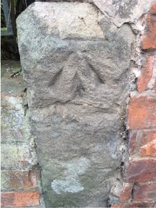
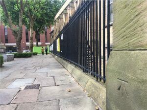
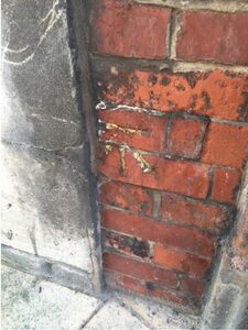
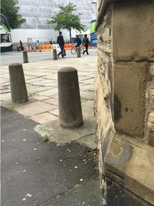
My colleague John Moore pointed out a couple of cut mark Ordnance Survey benchmarks on and around Oxford Road. This prompted me to look up the nearest benchmarks and find them. I’ll keep updating this post as I photograph them – some are currently off-limits because of building work, others have likely been destroyed. These marks are a legacy of a need for marks for local surveyors using optical levels, alidades, chains and plane tables – these marks are no longer maintained by the Ordnance Survey. A modern surveyor will use a GPS receiver that uses a correction signal from a receiver located on a known position – the organisation provides an “active” network of continuously running transceivers on known positions, and a “passive” network of survey marks with published positions upon which a surveyor may locate their own transceiver.

 

 

 

 

 

• SJ84849678, Number 81 Upper Brook Street, north-west face, west angle. 38.868m O.D. – No longer extant.
• SJ84579662, Museum, west side Oxford Road, south side gateway, north-east face, north angle. 38.384m O.D. Obscured by building works at present.

Because loss-on-ignition (L.O.I) can be so time consuming in routine analysis of soils, peats, lake or marine sediments, we’ve been testing a CEM Pheonix microwave furnace as a substitute to the old muffle furnace methods.

Determining Ramp, Cooling Times and Batch Sizes

The muffle furnace takes around 45mins to get to 550deg.C, and cooling is a three-step process, where the furnace cools naturally to around 250deg.C, then transferring the crucibles to a heat sink plate to cool to 50deg.C, then transferring to a desiccator until room temperature for weighing. This three-step process takes about an hour and a half to two hours. A single batch in the muffle furnace consists of 64 samples.

The microwave furnace takes around 20mins to get to 550deg.C, and cooling is pretty much instant because of the quartz fibre crucibles. A single batch is up to 15 samples.

Determining Ignition Time

For loss-on-ignition, the standard ignition time is 2 hours. For the microwave furnace, I performed a test to determine the most appropriate time, using a mixed peat that had been powdered and dried overnight at 105deg.C. Sample sizes were around 0.3g dry weight.

5mins = 95.4% L.O.I @ 550deg.C – the sample was observed to be igniting when removed from the furnace

10mins = 95.8% L.O.I @ 550deg.C

20mins = 96.4% L.O.I @ 550deg.C

30mins = 95.4% L.O.I @ 550deg.C

60mins = 96.5% L.O.I @ 550deg.C

Testing Comparability

As an initial test I tested the same peat used in the test above, with three repeats. Sample sizes were around 0.7g dry weight.

Muffle furnace = 95.165+/-0.09g L.O.I @ 550deg.C

Microwave furnace = 95.367+/-0.69g L.O.I @ 550deg.C

I’m planning further analyses to compare with results derived from elemental analysers, muffle and microwave furnaces, but these initial tests indicate the methods are likely to be comparable.

Conclusions

Both units provide comparable results. The muffle furnace has a total batch time of around 4hrs45mins, and a maximum batch size of 64, whereas the microwave furnace has a batch time of under 35mins, and a batch size of 15, so a 64 samples could be analysed in under 3hrs. The microwave furnace has the added advantage of integrated balance and L.O.I calculations, and fewer hot surfaces, particularly when using the recommended quartz fibre crucibles. There is no reason why the microwave method wouldn’t be suitable for ignitions of 950deg.C for estimating inorganic carbon content.

I’ve added a new poster of a stereomicroscope to my previous post on microscope diagrams for the lab.

Microscope Teaching Resources

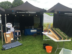
This weekend I joined a crew from Geography at the University of Manchester for the Bluedot Festival at Jodrell Bank, exhibiting some of our work on the local ecology and quaternary history, with a particular emphasis on upland environments. Along with other exhibitors, our stall was busy all weekend, and I met hundreds of interesting people enjoying the exhibits, lectures and music.

The format of music festival with science outreach (activities, lectures, stand-up, installation art etc.) works brilliantly, and I hope it runs again (update – it is!). The atmosphere was relaxed, with conversations about science projects between visitors over good food and drink all over the site. On a side note I’ve never encountered a more considerate audience – visitors and staff made a special effort to make the event work for families as well as the usual festival crowd, and make the most of what the exhibitors and artists had to offer.

I’ve been reading around some other blogs and although generally positive, I can’t help thinking some folks have missed the point a bit. Amy Parkinson’s blog on the University of Manchester website, while positive, focusses solely on the music and doesn’t mention the scores of University of Manchester staff and students in the “Star Field” exhibition area, or any of the lectures given by University staff, students and alumni (for example, the excellent Katie Steckles, who can and does make folding paper interesting!) The MEN article focusses on a certain Lee Taylor who reckons he once smelt someone smoking something illegal, and their other reviews again focus on the music, totally missing the science angle on all this – The Guardian are just as guilty.

So, to redress the balance – there were two large, full tents with short talks and lectures throughout the weekend (I heard about parasitic gut creatures, and watched electrical stimulation used to “remotely control” a body, amongst other things), and visited exhibits on meteorites, saw hardware from the Hubble Space Telescope, while in other displays young people were building robots and learning about allergies. There were lecturers and professors with their undergraduate and postgraduate students, chatting away with parents while kids tried out the interactive displays, while others were answering those science questions people “always wanted to ask” or just chatting about life as a scientist.

Last month I took my Amateur Radio Foundation Licence exams, and Ofcom have now granted me a call-sign, M6TKG. I’m planning on taking my intermediate exams early next year, but for now I’m going to explore some mobile analogue voice and digital text modes, alongside my existing interests in decoding ACARS and ADS messages used in aviation. As I found myself doing more and more diagnostic work on drones (2.4GHz digital, bluetooth, WiFi, GNSS), telemetry (GSM), emergency beacons (406MHz) and satellite telephony (SPOT, Iridium), I thought I should improve my working knowledge of radio. Amateur radio is actually really rewarding, and a practical way to learn about electronics and radio. It was a generous leaving gift from the staff in Geography at The University of Southampton that enabled me to buy the course texts and my first radio transceiver –  thanks!