Author: Tom Bishop

It’s always nice to be name checked in papers where we’ve been involved in lab or field work, and it’s even better when it’s a great paper in a top journal! For this work we assisted in the methodological development of the microplastic extraction procedure. Microplastic extraction is a complex and time-consuming process involving density separation of the material in a sample, and the nature of the sediment and depositional context and process needs careful consideration.

Kane, I. A., Clare, M. A., Miramontes, E., Wogelius, R., Rothwell, J. J., Garreau, P. and Pohl, F. (2020). Seafloor Microplastic Hotspots Controlled by Deep-Sea Circulation. In Science 30 April 2020. DOI: 10.1126/science.aba5899

I’ve recently worked on a piece with Technicians Make it Happen about the work I’m doing while the university campus is closed. You can read it here.

Introduction

The Raspberry Pi is a small-format computer that can run a number of general purpose operating systems, the most popular of which is a build of Linux.

Most computers have relatively poor in-built timekeeping. A time server reads a reference clock and distributes that information over a network. Most computers that have an internet connection regularly synchronize from a publicly accessible timeserver over the internet without the user even knowing.

Accurate timekeeping is important for a number of computing applications; for amateur radio operators using digital modes like JT-X, it is essential to the correct operation of the mode. This blog post explains how I used a cheap GPS chip and Raspberry Pi to serve time to my home network.

Choosing the GPS Chip

The global positioning system is familiar to many as a constellation of orbiting satellites that provides positioning information, but at the heart of each satellite is an atomic clock – the entire system works by comparing slight differences in the time it takes signals from 3 or more satellites to reach a receiver. If you can pick up a signal from a GPS satellite, you have the output from a precise atomic clock, and this can be used to “discipline” (synchronize) your timekeeping.

Most GPS chips pass a message every second containing positioning, diagnostic and timing information. Because this message always arrives slightly (and unpredictably) late, some GPS chips can also supply another channel that pulses to precisely mark the beginning of every second (pulse-per-second, or PPS), a bit like the “pips” on the radio. Obviously the two sources of information need to be combined, as the PPS doesn’t tell the time or date, only the beginning of each second.

You will need a GPS chip that has a serial output, and ideally a pulse-per-second (PPS) output. I used a very cheap (£7 delivered) board from China called a “Beitian BS-280”, which has an integral antenna and a U-BLOX G7020-KT GNSS receiver. It has 6 I/O connections:

• Tx: TRANSMIT, the channel on which serial data is transmitted from the GPS to the Raspberry Pi
• Rx: RECEIVE, the channel on which serial data is received by the GPS from the Raspberry Pi
• GND: GROUND connection
• VCC: POWER connection for the GPS, typically 5v
• PPS: PULSE-PER-SECOND timing signal
• U.FL: optional external antenna connection

Initial Configuration of the Raspberry Pi

I’ll assume a certain familiarity with Raspberry Pi and/or Linux, so I will refrain from offering a complete step-by step guide to the initial configuration of the Raspberry Pi, as there are many guides available on the internet. I will say that I installed a minimal version of Rasbian 10 (Buster), expanded the filesystem, configured a WiFi connection to my home network using wpa_supplicant and ran the usual updates. The entire configuration was performed via a remote SSH connection.

Connecting the GPS Chip

Firstly, make the following connections between the Raspberry Pi and the GPS:

• RasPi Pin 10 <-> GPS Tx
• RasPi Pin 8 <-> GPS Rx
• RasPi Pin 4 <-> GPS Vcc
• RasPi Pin 6 <-> GPS Gnd
• RasPi Pin 7 <-> GPS PPS

Remember to position your GPS antenna somewhere it can receive a signal – normally with a direct line-of-sight to a sky view. My GPS receiver performs very well in the loft, with the antenna facing the sky.

Next we need to configure the Raspberry Pi to listen to the GPS on the serial interface. By default the Raspberry Pi has a terminal setup on those pins, so we need to run sudo raspi-config and enable to serial connection, and disable the serial console. You can check the interface is now working by running cat /dev/serial0 or cat dev/ttyS0. You should see NMEA formatted data. If you see new data appearing every second, everything is working.

Next we must check that the PPS signal is working correctly. On my unit, the PPS signal is also linked to a LED on the unit, so it is easy to tell when a PPS signal is being produced. To check it is being received:

1. Install software using sudo apt-get install pps-tools.
2. Add the line dtoverlay=pps-gpio,gpiopin=4 to the bottom of /boot/config.txt.
3. Reboot, and check the output of sudo ppstest /dev/pps0; you should see a line every second.

Setup Timeserver Software

Disable NTP in DHCP

In order to run the Raspberry Pi as a timeserver, we first need to stop it trying to look for another timeserver to syncronise with!

1. Remove ntp-servers from /etc/dhcp/dhclient.conf.
2. Delete /lib/dhcpcd/dhcpcd-hooks/50-ntp.conf

Install GPSD

Next we install the software that parses the information from the GPS chip and makes it accessible for the time server software.

1. sudo apt-get install gpsd-clients gpsd
2. Edit /etc/default/gpsd as follows:

# /etc/default/gpsd
#
# Default settings for the gpsd init script and the hotplug wrapper.

# Start the gpsd daemon automatically at boot time
START_DAEMON="true"

# Use USB hotplugging to add new USB devices automatically to the daemon
USBAUTO="false"

# Devices gpsd should collect to at boot time.
# They need to be read/writeable, either by user gpsd or the group dialout.
DEVICES="/dev/serial0 /dev/pps0"

# Other options you want to pass to gpsd
#
# -n    don't wait for client to connect; poll GPS immediately

GPSD_OPTIONS="-n"

3. Now the moment of truth – test it with gpsmon. You might need to use set term=vt100 if it looks odd. This should display both GPS position (latitude and longitude),and a number next to “PPS”.
4. It needs to be setup to boot at background, so use:
   • systemctl daemon-reload
   • systemctl enable gpsd
   • systemctl start gpsd
5. Test the system by rebooting and immediately checking sudo ntpshmmon. You should see the two sources.

Setup the Time Server

1. Check that both time sources are being seem in sudo ntpshmmon.
2. Install NTP with sudo apt-get install ntp.
3. Modify/etc/ntp.conf by adding the lines:

# GPS PPS reference
server 127.127.28.2 prefer
fudge  127.127.28.2 refid PPS

# get time from SHM from gpsd; this seems working
server 127.127.28.0
fudge  127.127.28.0 refid GPS

4. Restart with systemctl restart ntp.
5. Check with ntpq -p. Please note, if you run this command a few times for the course of an hour or so, you’ll see things change quite a bit.
6. Eventually, you’ll want to see the PPS (.SHM.) as the * (selected for synchronization), probably the GPS removed (x or -) and a few random servers in the mix (+) as well. There’s lots of information out there on how ntp decides what the time is by combining multiple sources.

Use the Timeserver

Having a timeserver on the network isn’t much use if your computers don’t know its there! On some network routers with DHCP you can define the server using the internal IP Address (you should also bind the MAC address of the Raspberry Pi to a fixed IP address!), or you can define the address of the server in your operating system settings.

Our Wolman Plate didn’t return from its last expedition, so I looked around for a replacement and was quite surprised to see just how much distributors will charge for what is essentially a thin sheet of aluminium with some holes in. Combined with some long lead times and with the next job looming, I made my own!

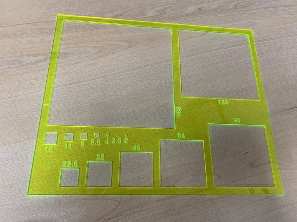
Many thanks for the B.15 Architecture Workshop for the use of their laser cutter. They cut my design from high visibility 3 mm Perspex sheet. You can cut your own from my AutoCAD files if you have access to a laser cutter, or order online from a manufacturer using the same file if not.

For more details on measuring coarse stream beds, start with the classic papers like Wolman (1954) and Leopold (1970).

Configuration of the UGGA

The UGGA is relaively simple to configure – simply turning the instrument on will begin measurement and recording. The status of the instrument can be checked using a laptop or tablet computer. Download a copy of a VNC terminal program, connect to the WiFi network broadcast by the instrument (SSID and password printed inside the instrument), and connect using the IP address, username and password in the manual. This will give access to the diagnostic screens.

At this point I recommend making a record of any offset between the UGGA clock and local time.

Configuration of the eosMX

Click on the top menu bar to minimise the LGR UGGA monitoring software, and open the Eosense multiplexer control software. Use the dialogue to test the chambers mechanical operation and program the required cycle, and start the process. The cycle events and data from any connected sensors will be recorded.

Importing Data into eosAnalyze

1. Place the UGGA recording file (gga_YYYY-MM-DD_fnnnn.txt) and the eosMX logfile (FRMonitor_nnnn.log) in the same folder as the software (eosAnalyze-AC_v3.6.2.exe).
2. Open the software and in the menu Data > Analyzer Data Path set the location to the location of the software (eosAnalyze-AC_v3.6.2.exe).
3. Toggle the Options > Toggle European Timestamp options so it is set to American timestamp format.
4. Ensure that the LGR UGGA is selected in Options > Equipment > Select Analyzer Type.
5. Ensure that Eosense eosAC (Multiplexed) is selected in Options > Equipment > Select Chamber Type.
6. The default values in Options > Equipment > Chamber/Analyzer Settings are usually acceptable, but if you have modified the system, you may need to change them.
7. If you have connected the auxiliary sensors, you must configure them in Options > Equipment > Configure Auxiliary Sensors. We have Decagon MAS-1 and RT-1 instruments available.
8. Now click on Collect Data and set the time range for your required measurements. I recommend setting a time range larger than the experiment duration so no data is truncated.
9. If the process has been successful, you will see measurement records appear in the Measurements window. Double click on one of the measurement records to bring up the Measurement Settings dialogue.
10. Modify the lower and upper deadbands (shown on the graph in green and red respectively) by changing the Data Domain values. Try to exclude the obviously bad data at the beginning and end of the measurement duration. Select Apply Deadband Range To All and OK to apply these parameters to all of the measurements.
11. To export the processed data, select Data > Export Data Table and select a location for the data file.

I’ve received a few queries recently that really boil down to a misunderstanding of the differences between tabular data formats and spreadsheets, so I thought I’d write a quick guide around the subject.

Delineated Text

These are more commonly known as “comma-separated values” (*.csv) or “tab delineated values” (*.tab), but are simply text files that describe a table. Usually, each line forms a row, and the value in each column is separated by some symbol (delineation), like a comma (,), semicolon (;) or a tab. Unfortunately, there is no standard definition of delineated text tables, but fortunately the parameters can usually be worked out. The key things to work out are:

• delineation between values (comma, semicolon, tab etc.)
• presence or absence of headers in the first row
• whether quotation marks (“”) are used to surround each field, or only where text is present
• what type of decimal point is used (usually a point (.) but occasionally a comma (,)
• the encoding of the text file (e.g. UTF-8)

This is my preferred format – it is minimal, platform-independent and supported by all major databases, programming languages, statistics packages and spreadsheet applications. See below for an example of delineated tabular data that uses commas to separate values, quotation marks around text, decimal points, and has a header row. In R you can create your own example using write.csv(head(iris), file = "iris.csv").

"","Sepal.Length","Sepal.Width","Petal.Length","Petal.Width","Species"
"1",5.1,3.5,1.4,0.2,"setosa"
"2",4.9,3,1.4,0.2,"setosa"
"3",4.7,3.2,1.3,0.2,"setosa"
"4",4.6,3.1,1.5,0.2,"setosa"
"5",5,3.6,1.4,0.2,"setosa"
"6",5.4,3.9,1.7,0.4,"setosa"

Spreadsheets

The two Excel spreadsheet data formats are *.xls and *.xlsx. These formats are technically very different, but functionally serve a similar purpose. Not only are tabular data stored (often multiple sheets), but formatting, formulae, and other metadata. For the purposes of data import and export, we are usually only interested in the cell values, so all of this extra data only serves to complicate the process. Spreadsheets are fundamentally different from tabulated data.

The Microsoft Excel Spreadsheet (*.xls) is a proprietary binary data format. Many other software packages have implemented this format based on the documentation released, but Excel now support the Microsoft Excel Open XML Format (*.xlsx).

This format is based on extensible markup language (*.xml), a well-defined way of creating structured documents that are both machine and human-readable. A number of these files sit within a folder structure that defines different spreadsheets etc., and the entire collection is then compressed (zipped) for efficiency and convenience. See below for an example of the code in an Excel Open XML sheet (created in R using the openxlsx library, e.g. write.xlsx(head(iris), file = "iris.xlsx").

<?xml version="1.0" encoding="UTF-8" standalone="yes"?><worksheet xmlns="http://schemas.openxmlformats.org/spreadsheetml/2006/main" xmlns:r="http://schemas.openxmlformats.org/officeDocument/2006/relationships" xmlns:xdr="http://schemas.openxmlformats.org/drawingml/2006/spreadsheetDrawing" xmlns:x14="http://schemas.microsoft.com/office/spreadsheetml/2009/9/main" xmlns:mc="http://schemas.openxmlformats.org/markup-compatibility/2006" mc:Ignorable="x14ac" xmlns:x14ac="http://schemas.microsoft.com/office/spreadsheetml/2009/9/ac"> <dimension ref="A1"/> <sheetViews><sheetView workbookViewId="0" zoomScale="100" showGridLines="1" tabSelected="1"/></sheetViews> <sheetFormatPr defaultRowHeight="15.0"/><sheetData><row r="1"><c r="A1" t="s"><v>0</v></c><c r="B1" t="s"><v>1</v></c><c r="C1" t="s"><v>2</v></c><c r="D1" t="s"><v>3</v></c><c r="E1" t="s"><v>4</v></c></row><row r="2"><c r="A2" t="n"><v>5.1</v></c><c r="B2" t="n"><v>3.5</v></c><c r="C2" t="n"><v>1.4</v></c><c r="D2" t="n"><v>0.2</v></c><c r="E2" t="s"><v>5</v></c></row><row r="3"><c r="A3" t="n"><v>4.9</v></c><c r="B3" t="n"><v>3</v></c><c r="C3" t="n"><v>1.4</v></c><c r="D3" t="n"><v>0.2</v></c><c r="E3" t="s"><v>5</v></c></row><row r="4"><c r="A4" t="n"><v>4.7</v></c><c r="B4" t="n"><v>3.2</v></c><c r="C4" t="n"><v>1.3</v></c><c r="D4" t="n"><v>0.2</v></c><c r="E4" t="s"><v>5</v></c></row><row r="5"><c r="A5" t="n"><v>4.6</v></c><c r="B5" t="n"><v>3.1</v></c><c r="C5" t="n"><v>1.5</v></c><c r="D5" t="n"><v>0.2</v></c><c r="E5" t="s"><v>5</v></c></row><row r="6"><c r="A6" t="n"><v>5</v></c><c r="B6" t="n"><v>3.6</v></c><c r="C6" t="n"><v>1.4</v></c><c r="D6" t="n"><v>0.2</v></c><c r="E6" t="s"><v>5</v></c></row><row r="7"><c r="A7" t="n"><v>5.4</v></c><c r="B7" t="n"><v>3.9</v></c><c r="C7" t="n"><v>1.7</v></c><c r="D7" t="n"><v>0.4</v></c><c r="E7" t="s"><v>5</v></c></row></sheetData><pageMargins left="0.7" right="0.7" top="0.75" bottom="0.75" header="0.3" footer="0.3"/><pageSetup paperSize="9" orientation="portrait" horizontalDpi="300" verticalDpi="300" r:id="rId2"/></worksheet>

Work with Delineated Text

It is clear from the examples given that for tabulated data, delineated text is preferable for both compatibility and efficiency. For more complex data (e.g. multivariate time series, or geo-referenced multivariate data), Network Common Dataform (NetCDF) is often preferable. Only where work needs to be done within Excel, Numbers or Sheets, and contains formulae or formatting, should spreadsheet formats be used.

I passed my final amateur radio exam, so I now have a full licence and callsign M0TKG (I’ve surrendered my old signs 2E0TKG and M6TKG). I’ll be running a little portable low-power (QRP) HF station and will also be active on the 6M, 2M (VHF) and 70CM (UHF) bands in south Manchester. I’m also thinking of taking my Morse exam, but we’ll see!

Need to draw a neat looking soil texture diagram? The soiltexture app in R is really powerful. For those in a hurry for coursework, I’ve made a little web app available here, but for those doing more advanced work, I’d recommend having a look at Julian Moeys guide to the package here.

Many of our lab users have been trying to use various Zeiss software packages to make measurements from photomicrographs. It is often easier and quicker to use ImageJ to make these measurements.

Here’s how:

Image Acquisition

1. Use the Zeiss Zen to acquire an image of a graticule or rule under the magnification settings you will using for your imaging.
2. Acquire the images you need.
3. Save the images in the Zen software as JPEG or TIFF files. Remember, keep your filenames and folder structure organised!

Calibrating the Scale

1. Open the ImageJ software. Open the image of the graticule or rule by selecting File > Open…
2. Using the line tool (5th button from the left), select two points of known distance. It is best to use the widest possible two points for best accuracy (e.g. if you can see 2 mm of marks in the image, don’t select only 1 mm mark distance). Use the zoom controls (10th from the left, then + and – keys) as required.
3. Click Analyze > Set Scale… and type the known distance (e.g. 2) in the second box down. Also, write the units (e.g. mm) in the appropriate box. Check the “Global” box to apply this to all images.
4. If you have changed the magnification, you can change the scale manually by adjusting the Known distance or Distance in pixels, but it is usually better to perform a new calibration for each magnification.

Making Measurements

1. Open the image file you wish to analyse using File > Open… or File > Open Next.
2. Select Analyze > Tools > ROI Manager.
3. Check the “Show All” and “Labels” boxes in the ROI Manager dialogue.
4. Using the straight line tool, select the edges of the object you want to measure. Press the [T] key or click the Add button in the ROI Manager.
5. Repeat until you have selected all of the objects you wish to measure.

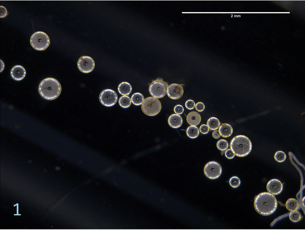
If you are measuring circular or oval objects, you may have better results using the oval selection tool (second from the left). You may wish to experiment with different selection tools depending on your measurement.

Exporting Data

1. When you have selected all of the objects you wish to measure, select “Measure” in the ROI Manager.
2. You may wish to obtain summary statistics – in this case, select Results > Summarize.
3. The Results dialogue will open. Save the data by selecting File > Save As…
4. If you name your file with a *.csv extension, you will be able to open it directly in statistics software of your choice.

Automated Analysis

You don’t have to select everything manually. The particles can be analysed automatically. Firstly, the colour image needs to be converted into binary. Then, individual particles need to be separated where they overlap, and finally, the automatic particle recognition can be run and summary statistics obtained.

1. Open the image file and ensure the scale is set correctly.
2. Open image > adjust > colour threshold and adjust the settings so that the particles are correctly picked out from the background. Set the Threshold colour to black & white.
3. Convert the image to black and white format by selecting Image > Type > 8-bit
4. If the particles have “holes” in, select Process > Binary > Fill Holes. You should see the particles fill.
5. To sort out overlapping particles, select Process > Binary > Watershed. You should see small white lines between all the particles.
6. Select Analyze > Analyze Particles. You may need to adjust the size range to eliminate objects that are not of interest. Note the size is expressed in mm^2, so for circular objects you’ll need to convert using area = 3.14 * diameter/2. The lower end of the circularity setting can also be adjusted for optimum results. For the example image I’ve used a size range of 0.01-4mm^2 and a circularity of 0.6-1.
7. In the show menu, select “Ellipses”.
8. Select “Add to manager”, “Exclude on edges”, and use “Display results”, “Clear results” and “Summarize” as required.
9. You can manually delete or add ellipses using the ROI Manager.

Other Tools

There’s loads of useful tools in ImageJ, including many that can speed up and improve repetitive workflows, and assist in preparing images for publication. Just pop by the office for a chat if you are interested in a demonstration of some features.

I’ve just passed my intermediate amateur radio exams with the help of Stockport Radio Society G8SRS. I’ll be keeping my previous call-sign M6TKG for now, but I’ll also now be using 2E0TKG under certain circumstances. As a gift to myself for passing, I’ve started putting together a little portable rig for low-power (QRP) work based on a Yaesu FT-817ND. I’ve already started reading for my full licence test, and have just begun working towards my 12 words-per-minute Morse code test. I hope that soon I’ll be in a position to bring a rig away when I travel, and make some contacts from some of the unusual places I sometimes have the opportunity to visit.